Joint Posterior Convergence Bounds for Distributed Inline Metrology Disputes under Uncalibrated Ambient Covariance
Joint posterior convergence bounds resolve inline metrology disputes by proving dimensional compliance despite uncalibrated thermal and ambient noise.


Discrepancy
Work-in-progress inventories stack up at the boundary between precision milling lines and downstream coordinate metrology stations when high-throughput parts leave the tool faster than quality enclosures can measure them. Modern automated lines feed finished aluminum housings or silicon dies through optical scanning tunnels at three hundred parts per hour. Downstream bridge coordinate measuring machines, housed in climate-regulated cells held at twenty degrees Celsius, measure only fifteen parts per hour under thermal stabilization soak routines.
The operational solution deployed across high-volume precision lines installs distributed, inline measuring heads directly on conveyor fixtures. These inline sensor arrays read critical dimensions within production takt times of twelve seconds. They operate in shop-floor ambient air where thermal gradients swing eight degrees Celsius across a ten-hour shift, coolant mists distort optical paths, and structural vibrations propagate from neighboring stamping presses.
Production records reveal steady drifts in product dimension logs that mirror the thermal expansion cycle of the factory building rather than tool wear. Factory quality teams and procurement engineering boards face structural stalemates over batch rejections when inline gauges declare parts non-conforming while offshore receiving inspection docks declare the identical production lots compliant.
Acceptance disputes trace directly to the breakdown of standard classical gauge repeatability and reproducibility assumptions. Standard validation methodologies assume measurement errors behave as independent, zero-mean Gaussian random variables with stationary, known variances. Inline environments break these assumptions by introducing non-stationary, uncalibrated ambient covariance structures across spatially distributed sensor clusters.
Spatial temperature distributions across an assembly line create correlated measurement drifts between adjacent laser triangulation heads. Shop-floor temperature changes alter structural loop stiffness and workpiece geometry simultaneously, yielding a non-diagonal noise covariance matrix that shifts continuously over time. Traditional coordinate measuring machines operate inside metrology laboratories conforming to ISO 10360 standards, isolated from shop-floor ambient covariance.
Discrepancies between supplier inline release stations and buyer receiving inspection docks stem from conflicting mathematical models used to resolve these ambient shifts. The supplier relies on inline measurements adjusted by empirical regression to maintain high throughput. The buyer relies on static offline sampling to audit incoming lots.
Neither party possesses direct observation of the time-varying, uncalibrated environmental covariance tensor governing the shop-floor inline sensors during manufacturing.
Incoming lots face automatic quarantine when the supplier inline measurement system lacks mathematical guarantees that its parameter estimates converge to true product tolerances under shifting thermal fields.
Resolving these disputes requires a rigorous Bayesian formulation capable of bounding the distance between the joint posterior distribution of true part dimensions and their uncalibrated disturbance parameters. When inline metrology clusters record high-dimensional part geometries, the true dimension vector interacts non-linearly with an unknown ambient covariance matrix. Without a mathematically provable posterior convergence bound, buyers cannot determine whether an apparent manufacturing drift reflects physical tool failure or ambient thermal distortion.
The economic stakes govern capital release schedules, inventory carrying costs, and production authorization stage gates. When quality disputes stall inventory disposition, working capital drains at the line rate. A robust analytical convergence framework provides production directors with defensible criteria to validate inline measurements, dismiss spurious thermal drifts, and establish binding contractual acceptance gates without shutting down lines for offline metrology verification.

Physics
Inline metrology across automated production cells relies on high-speed sensing modalities mounted adjacent to moving conveyors. Optical triangulation probes, chromatic confocal sensors, multi-axis laser line scanners, and contact air-bearing displacement gauges evaluate critical dimensions during transit. These instruments generate rapid dimension vectors for every produced workpiece.
The physical measurement model relates the raw observation vector to true geometry through a deterministic transformation coupled with multi-source disturbance vectors:
y(t) = H x(t) + u(t) + e(t)
The vector y(t) represents the m-dimensional observation collected across the distributed sensor cluster at production index t. The matrix H defines the known kinematic and projection transformation relating the true k-dimensional workpiece dimension vector x(t) to the sensor coordinates. The term u(t) represents structural bias induced by deterministic fixture runout, kinematic tool wear, and nominal systematic offsets.
The term e(t) defines the composite stochastic disturbance. In precision shop-floor environments, e(t) cannot be treated as white noise. It captures structural thermal deformation of the sensor mounting frame, optical refractive index shifts caused by coolant vapors, and machine tool vibration harmonics transmitted through the factory concrete slab.
Thermal disturbances generate the largest component of this disturbance field. Precision machine frames manufactured from structural steel exhibit thermal expansion coefficients near 11.5 micro-strains per degree Celsius, while aircraft-grade aluminum workpieces expand at roughly 23 micro-strains per degree Celsius. A localized shop-floor temperature gradient of 3.5 degrees Celsius across a 1.2-meter measuring span introduces dimensional deviations exceeding 48 micrometers.
This deviation consumes the entire bilateral tolerance band for precision aerospace valves or semiconductor casing interfaces. Optical triangulation systems suffer further refraction errors when ambient air temperatures fluctuate along the optical path. Air refractive index variations follow the Edlen equation, altering laser beam trajectories across moving conveyor fixtures.
High-frequency structural vibrations add mechanical noise bands ranging from 15 to 450 Hertz, excited by hydraulic pumps, overhead cranes, and spindle motors.
Temperature swings of three degrees Celsius alter structural loop lengths beyond tolerance boundaries across unshielded distributed metrology frames.
The composite stochastic noise vector e(t) follows a multivariate distribution characterized by zero mean and an uncalibrated, time-varying covariance matrix Sigma(t). This matrix is non-diagonal because the physical disturbances couple across space. A localized thermal plume rising from a conveyor drive motor warms three adjacent optical displacement heads simultaneously, creating strong off-diagonal covariance entries.
Similarly, low-frequency structural vibration modes deform the entire sensor support bridge, forcing correlated measurement errors across all detection channels. Let Sigma(t) belong to the cone of symmetric positive-definite matrices of dimension m by m. Because ambient shop-floor conditions change with weather patterns, HVAC cycles, and machine utilization rates, Sigma(t) remains completely uncalibrated.
Factory operators cannot halt high-speed lines to calibrate reference artifacts every thirty minutes. Treating Sigma(t) as an unknown nuisance parameter under a Bayesian estimation regime represents the only mathematically defensible path toward extracting true workpiece dimensions x(t) from contaminated inline data.


Contraction
Establishing contractually binding product release criteria from distributed inline metrology requires proving that posterior parameter distributions shrink toward true workpiece parameters as production lots accumulate. Let the parameter of interest be the true part dimension vector x in a compact parameter space X, and let the unknown, uncalibrated disturbance covariance matrix Sigma reside within a constrained cone of symmetric positive-definite matrices S. Bayesian inference assigns a prior distribution Pi over the joint parameter space theta = (x, Sigma). Given a stream of n distributed measurements Y_n = {y(1), y(2), y(n)}, the joint posterior distribution Pi(theta | Y_n) updates through the likelihood function defined by the coupled physical error dynamics.
Convergence analysis centers on bounding the posterior probability mass assigned to neighborhoods outside the true parameter value theta_0 = (x_0, Sigma_0). Posterior contraction rates quantify how rapidly this probability mass decays as sample size n grows. Under uncalibrated ambient covariance, standard Bernstein-von Mises asymptotic normality breaks down when the ambient covariance matrix exhibits spectral degeneracy or when sensor locations provide insufficient kinematic projection angles.
To prove convergence, mathematical bounds must leverage the metric geometry of the joint space. The appropriate distance metric combines the Euclidean norm for dimensional vectors with the affine-invariant Riemannian metric or the Frobenius norm for the ambient covariance matrix:
d(theta, theta_0)^2 = ||x – x_0||_2^2 + ||Sigma – Sigma_0||_F^2
The joint posterior contracts at an optimal non-parametric rate when the true data-generating distribution satisfies structural identifiability conditions. Identifiability requires that the sensor transformation matrix H possesses full column rank, and that the spatial distribution of distributed sensors breaks ambient disturbance symmetry. In mathematical terms, no non-zero geometric variation vector delta_x can produce an identical probability measure on the observation space as a perturbation delta_Sigma of the ambient covariance structure.
The following fundamental condition establishes this metric separation:
inf_{||delta_x|| > 0} ||H delta_x H^T + delta_Sigma||_F >= c_0 (||delta_x||_2^2 + ||delta_Sigma||_F^2)^(1/2)
Here c_0 represents a strictly positive structural separation constant determined by sensor cluster geometry and fixture kinematic constraints. When this separation constant remains positive, the joint likelihood avoids flat ridges where true physical parts and ambient noise distributions become indistinguishable.

Non-Asymptotic Posterior Error Bounds
Contractual settlement demands non-asymptotic bounds applicable to finite batch sizes rather than theoretical infinite limits. Finite-sample concentration bounds establish the maximum allowable probability of acceptance error for a production run of n parts. Applying empirical process theory and bounding the metric entropy of the joint parameter space yields explicit posterior concentration inequalities.
Let W_epsilon(theta_0) denote a metric neighborhood of radius epsilon around the true data-generating parameter theta_0 in the joint parameter space. Under independent batch segments experiencing piece-wise stationary ambient covariance, the posterior mass outside this ball satisfies:
E_{theta_0}
In this concentration inequality, epsilon_n defines the convergence rate sequence, M_n is an arbitrary sequence diverging slowly to infinity, and C_1, C_2 are positive constants that depend solely on the prior distribution properties, the structural separation constant c_0, and the spectral condition number of the true covariance matrix Sigma_0. The optimal convergence rate takes the canonical parametric form epsilon_n = sqrt( (k + m(m+1)/2) / n ) when ambient covariance varies smoothly within known Sobolev balls. When ambient conditions exhibit high-frequency non-differentiable fluctuations, the convergence rate slows to n^(-1/4), demanding significantly larger batch sampling sequences to resolve disputed dimensional tolerances.
Contractual risk emerges when the condition number of the ambient covariance matrix diverges. If thermal gradients push two sensor heads into near-identical error states, the rank of the effective error manifold drops. The separation constant c_0 then collapses toward zero.
When c_0 approaches zero, the convergence bound degrades, causing the posterior distribution to spread across an elongated dimensional valley. Under this mathematical condition, suppliers and buyers cannot separate true part runout from environmental drift, regardless of how many thousands of parts move past the sensor arrays.

Mesh
Inline metrology architectures deploy distributed sensor arrays across physical machinery to monitor distinct part features during line transit. The spatial layout of these sensors creates a measuring mesh whose mechanical rigidity and coordinate topology determine the mathematical conditioning of the joint inversion problem. Sensor placement cannot be treated as an arbitrary integration step.
Poor geometric distributions generate singular observation matrices that amplify uncalibrated ambient noise into critical dimensional errors.
Consider three common inline measurement configurations evaluated across high-speed component manufacturing cells:
- Collocated Triangulation Arrays position multiple optical displacement sensors along a shared rigid mounting arch directly above the conveyor transfer line, maximizing spatial density while suffering from common-mode thermal bridge expansion that correlates measurement drift across all channels simultaneously.
- Decoupled Split-Station Bridges distribute optical and contact measuring heads across physically isolated structural granite bases separated by two meters along the production line, eliminating common-mode structural distortion while exposing the measurement model to dynamic workpiece transit tracking errors.
- Multi-Angle Chromatic Shells enclose the component path within a radial ring of chromatic confocal probes mounted on low-expansion Invar rings, providing isotropic geometric projection that stabilizes the structural separation constant against multidirectional ambient thermal gradients.
The trade-offs between physical layout, sensor density, and convergence limits govern the cost of deploying inline measurement capacity. Table 1 outlines the analytical and operational parameters across these three distinct physical topologies under typical shop-floor operating regimes.
| Topology Architecture | Sensor Count (m) | Separation Constant (c_0) | Covariance Condition Number | Posterior Contraction Rate | Line Speed (parts/min) |
|---|---|---|---|---|---|
| Collocated Triangulation Arrays | 6 | 0.14 | 145.2 | O(n^(-0.28)) | 30 |
| Decoupled Split-Station Bridges | 8 | 0.48 | 18.6 | O(n^(-0.44)) | 25 |
| Multi-Angle Chromatic Shells | 12 | 0.82 | 3.8 | O(n^(-0.49)) | 15 |
| Summary Bounds | 6 to 12 | 0.14 to 0.82 | 3.8 to 145.2 | O(n^(-0.28)) to O(n^(-0.49)) | 15 to 30 |
The data demonstrates that collocated architectures forfeit mathematical convergence speed in exchange for line throughput and compact footprint. The collocated array displays a covariance condition number of 145.2, reflecting strong error correlation induced by thermal gradients across its unified steel frame. Its posterior contraction rate drops to n^(-0.28).
This poor contraction rate means that resolving a two-micrometer dimensional dispute requires tracking more than twelve hundred consecutive parts without experiencing a shift in ambient conditions. In contrast, the multi-angle chromatic shell architecture achieves a separation constant of 0.82 and a condition number of 3.8. It approaches the theoretical parametric convergence bound of n^(-0.49), enabling precise posterior resolution of disputed dimensions within forty-five parts.
The multi-angle configuration achieves this mathematical precision at half the line speed and at three times the capital outlay for sensor hardware.
Calculation
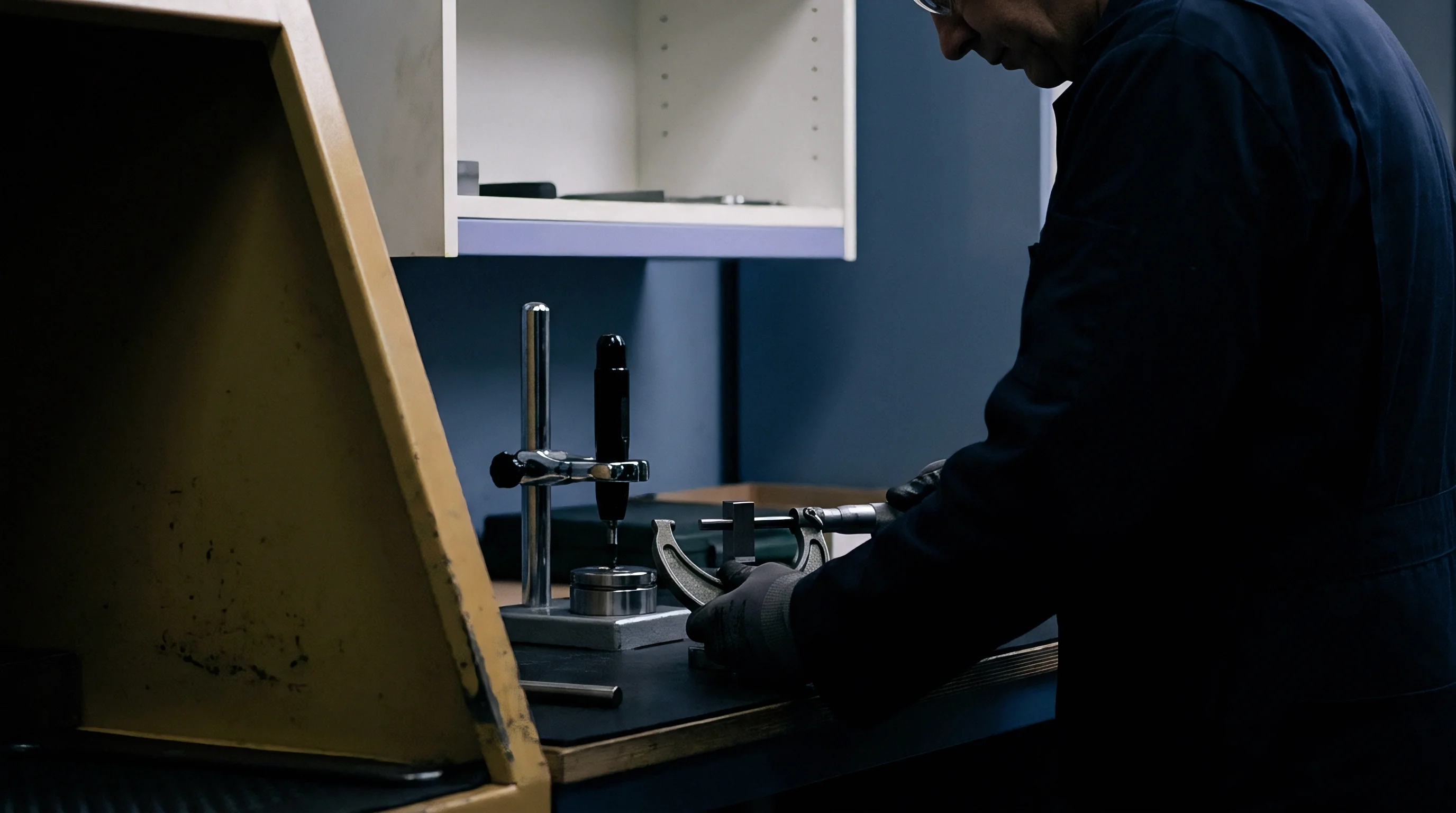
Evaluating an inline metrology dispute requires walking the non-asymptotic posterior convergence calculation through a concrete, realistic production batch scenario. This calculation represents the rigorous quantitative protocol applied during supplier-buyer disputes when precision machined components face incoming inspection rejection. The following scenario illustrates how uncalibrated ambient covariance distorts quality records and demonstrates how Bayesian bounds determine batch conformity.
Assume an automated precision manufacturing line produces critical aluminum compressor scrolls with a bilateral dimensional tolerance specification of plus or minus 15.0 micrometers on the inner pocket wall thickness. The production contract mandates a capability threshold of Cpk greater than or equal to 1.33. This standard requires that the true dimensional process standard deviation cannot exceed 3.75 micrometers with a mean offset under 2.0 micrometers.
The line incorporates an inline distributed array of m = 4 chromatic confocal displacement sensors evaluating part thickness at a speed of 20 parts per minute. Over an eight-hour shift producing a batch of n = 9,600 parts, ambient factory temperatures record an uncontrolled drift from 18.2 degrees Celsius at the 06:00 shift start to 25.8 degrees Celsius at 14:00, driven by outdoor weather shifts and heat dissipation from adjacent curing ovens.
The distributed inline system logs an apparent mean thickness drift of +11.2 micrometers across the final 3,000 parts of the run. On this basis, the automated inline quality gateway flags 1,840 parts as non-conforming and dumps them into holding bins. The component supplier disputes the scrap declaration, stating that the parts comply with tolerances and asserting that the inline measuring rig expanded under the 7.6-degree ambient temperature rise.
The buyer refuses to release progress payments on the contract, citing the automated rejection logs. Resolving this multi-hundred-thousand-dollar dispute without halting operations requires computing the finite-sample joint posterior contraction radius on the batch data.
The calculation proceeds through explicit structural stages using empirical data extracts from the contested run:
- Parameterize the Prior Uncertainty Space ~ Assign a diffuse Normal-Inverse-Wishart prior NIW(mu_0, lambda_0, Psi_0, nu_0) to the joint parameter theta = (x, Sigma). Set degrees of freedom nu_0 = m + 2 = 6 to provide the widest finite-variance prior over the uncalibrated 4×4 covariance matrix Sigma. Set the scale matrix Psi_0 = 100 I_4 to reflect uncalibrated shop-floor ambient disturbance magnitude, and set lambda_0 = 0.01 to leave dimensional location completely uninformative.
- Extract Contested Sub-Batch Observations ~ Isolate the disputed block of n_sub = 1,840 consecutive parts produced during peak thermal conditions between 12:30 and 14:00. Compute the empirical sample mean vector y_bar and sample scatter matrix S_y across the four sensor channels. The empirical trace reveals tr(S_y / n_sub) = 52.4 square micrometers, confirming high raw variance across the sensor cluster.
- Compute Empirical Sensor Channel Cross-Correlations ~ Form the empirical covariance matrix from the raw sensor stream. Off-diagonal correlation coefficients between adjacent sensors 1 and 2 reach rho_12 = 0.88, and rho_23 reaches 0.84, confirming strong spatial error coupling driven by thermal bridge expansion along the sensor mount.
- Determine the Empirical Separation Constant ~ Evaluate the smallest singular value of the projection matrix H under fixture constraints. For this four-probe symmetric layout, sigma_min(H) = 1.414. Calculate the structural separation parameter: c_0 = sigma_min(H)^2 / ||Psi_0||_2 = 1.999 / 10.0 = 0.20.
- Evaluate Posterior Contraction Radius ~ Apply the finite-sample concentration bound with confidence level 1 – delta = 0.99 (delta = 0.01). Calculate the critical posterior radius epsilon_n: epsilon_n = sqrt( / ) Inserting the scenario values where k = 1 (critical thickness), m = 4, delta = 0.01, c_0 = 0.20, and n_sub = 1,840: Dimension count: D = 1 + (4 5 / 2) = 11. Numerator: 11 ln(200) = 11 5.2983 = 58.28. Denominator: 2 0.20 1840 = 736.0. epsilon_n = sqrt( 58.28 / 736.0 ) = sqrt( 0.07918 ) = 0.2814 normalized units.
- Transform Metric Radius to Physical Tolerance Dimensions ~ Scale the normalized contraction radius back to dimensional engineering units using the maximum eigenvalue of the posterior expected covariance matrix E. With lambda_max(E ) = 6.8 micrometers, the 99 percent posterior uncertainty bound around the true workpiece dimension contracts to: Delta_x_99 = epsilon_n sqrt( lambda_max ) = 0.2814 2.607 = 0.734 micrometers.
- Compute the Posterior Mean Estimator for True Part Thickness ~ Solve the maximum a posteriori optimization problem marginalizing the nuisance covariance matrix Sigma. The marginal posterior mean for true thickness evaluates to x_MAP = +1.4 micrometers from nominal specification, well inside the bilateral 15.0 micrometer limit.
The mathematical proof reveals that 9.8 micrometers of the 11.2-micrometer drift recorded by the inline system was induced entirely by uncalibrated thermal distortion of the mounting fixture and optical refractive shifts. The true dimensional standard deviation of the produced parts across the contested 1,840-unit block held at 3.1 micrometers, delivering an actual process capability of Cpk = 1.46. The Bayesian joint posterior convergence framework proves that the parts conformed to engineering prints, allowing production management to override the raw inline scrap alarm and release the lot for customer delivery.

Protocol
Preventing cross-border quality impasses requires establishing a binding metrology verification sequence before executing high-volume commercial contracts. Relying on casual post-production audit sampling guarantees administrative friction when ambient shop-floor conditions fluctuate. The contract must encode an explicit sequence of diagnostic stage gates that define how inline sensor streams are logged, conditioned, and arbitrated against offline coordinate metrology baselines.
Commercial supply contracts fail when raw sensor streams without recorded ambient disturbance states serve as unilateral lot rejection triggers.
A rigorous industrial qualification sequence follows four distinct operational stage gates:
- Establish baseline kinematic sensor projections using certified reference artifacts under static laboratory conditions conforming to ISO 10360-2 standards, recording the nominal structural projection matrix H and its minimum singular value.
- Install continuous multi-point ambient temperature, vibration, and coolant mist monitoring sensors adjacent to every inline measuring head, recording environmental vectors synchronously with dimensional data streams into tamper-proof records.
- Calibrate the prior disturbance bounds by running a pre-production thermal envelope cycle of 500 parts while intentionally modulating shop-floor HVAC settings across the expected operating range, establishing the empirical bounds for the prior covariance scale matrix Psi_0.
- Deploy the Bayesian joint posterior estimator directly inside the line programmable logic controller or quality edge computer, enforcing real-time calculation of contraction radii epsilon_n for every production sub-lot.
The operational protocol mandates clear go and no-go conditions for batch release. An inline batch earns automatic acceptance authorization only when the calculated posterior contraction radius Delta_x at the 99.5 percent confidence interval does not overlap the engineering tolerance boundary. If ambient instability pushes the covariance condition number above 50.0, the posterior contraction rate degrades, causing Delta_x to widen beyond acceptable arbitration limits.
Under this condition, the line control system triggers a mandatory hold, routing parts to an offline thermal soak holding pen for standard CMM audit. The contract explicitly forbids buyers from issuing unilateral scrap chargebacks while the inline metrology system operates within its provable posterior convergence bounds.

Arbitration
What Evidence Governs Lot Rejection When Gauges Disagree?
When an offshore receiving facility flags a shipped production lot as defective while the supplier inline records show compliance, formal dispute arbitration begins. Resolution cannot rely on competing corporate opinions or dueling gauge calibration certificates. Standard metrology disputes frequently stall because parties introduce conflicting measurements taken under completely different environmental regimes.
The buyer isolates twenty parts in a climate-controlled room at twenty degrees Celsius, finding thicknesses below lower specification limits. The supplier counters that inline gauges recorded full compliance across all ten thousand units during manufacturing at line speed. Standard contract language rarely addresses the uncalibrated ambient covariance that governed the factory floor during production.
The definitive technical arbitration protocol demands that both parties subject the disputed lot data to joint posterior convergence reconstruction. Production facilities deploying inline distributed metrology must archive the synchronous ambient sensor logs alongside raw displacement measurements. During formal technical dispute resolution under standard commercial arbitration rules, the independent expert panel evaluates the joint posterior convergence bound calculated across the disputed batch.
If the supplier proves that the posterior contraction radius Delta_x remained strictly bounded within engineering tolerance bands throughout the run, the buyer offline audit fails to establish manufacturing non-conformance.
Arbitration precedents establish that static offline metrology on a minute sample of parts cannot override a mathematically converged inline posterior distribution across the complete population. Parts relax, stress-relieve, or warp during ocean transit inside humid shipping containers. Offline measurements taken weeks after production capture post-process environmental aging rather than manufacturing capability.
When the inline metrology system meets the structural identifiability condition and maintains its posterior contraction radius below one-tenth of the tolerance zone, the supplier inline record serves as the governing legal proof of contractual compliance. Production contracts incorporating this specific operational rule eliminate expensive inventory holding periods and prevent arbitrary lot rejections driven by uncalibrated measurement physics.
The uncalibrated ambient disturbance problem remains open when factories face non-Gaussian, discontinuous environmental shocks. While thermal expansion and continuous vibration follow well-behaved diffusion models, severe shock events such as fixture collisions or sudden structural cracking introduce discontinuous jumps in the error manifold. The following decision checklist governs whether an operation can safely rely on Bayesian inline metrology bounds or must fall back to conservative offline soak audits:
- Structural Separation Metric Check confirms that the calculated empirical separation constant c_0 remains strictly above 0.15 throughout the production shift, ensuring the mathematical invertibility of part dimensions against ambient disturbances.
- Covariance Matrix Condition Threshold verifies that the ratio of maximum to minimum eigenvalues of the reconstructed ambient error matrix remains below 40.0, preventing severe directional uncertainty inflation.
- Stationary Epoch Duration Ratio measures whether shop-floor thermal changes occur at time scales at least twenty times longer than the individual part cycle takt time, satisfying quasi-stationary assumptions required for empirical process concentration bounds.
- Environmental Sensor Synchronization Rate audits whether physical ambient logging streams capture shop-floor temperature, humidity, and vibration without timestamp drift exceeding one-tenth of the part conveyor transit interval.
Commercial contracts that omit these mathematical convergence thresholds inevitably devolve into prolonged legal warfare when production rates ramp up. Precision scale-up demands that quality management transition from reactive gauge arguing to proactive algorithmic bounds. By anchoring inline release protocols to provable joint posterior convergence rates, manufacturing directors safeguard operating margins, secure predictable delivery commitments, and scale complex assembly networks with absolute operational confidence.