Calculating Real Utility Demand to Prevent Voltage Sag and Air Pressure Losses
Calculate real utility demand using empirical millisecond-level coincidence vectors to size low-impedance feeders and local buffers, preventing voltage sags and air loss.

Draw
Nameplate power and continuous air ratings routinely deceive capital planning teams. Plants trip secondary distribution breakers or stall high-speed packaging actuators even with total utility capacity sitting fifty percent above average demand. The mistake stems from the arithmetic of coincidence and duration: steady-state averages mask sub-second spikes where electrical inrush and pneumatic valves draw at the exact same instant.
When twenty servo drives accelerate synchronized tooling while four twin-screw compressors cycle against unloader stages, dynamic utility load diverges completely from the shift-level meter log.
Sizing factory feeds properly requires separating connected load, nominal operational load, and peak transient coincidence. Engineers frequently pick arbitrary diversity factors between 0.6 and 0.8 across equipment schedules without empirical logging, but these lumped assumptions cover up localized bottlenecks. A cell of six automated stamping presses might carry a combined thermal rating of 400 kilowatts, yet during clutch engagement and hydraulic ram acceleration, dynamic draw reaches 1,100 kVA for 350 milliseconds.
When distribution transformers or feeders lack the low-impedance headroom to supply that transient current, terminal voltage drops sharply at the busbar.
A thirty-millisecond sag below seventy percent of nominal voltage collapses variable frequency drive DC links across adjacent automation cells.
Pneumatic systems show the exact same structural vulnerability. Compressor OEM documentation quotes free air delivery under steady test conditions governed by ISO 1217 Annex C, assuming an infinite supply basin and linear system resistance. Inside an operating cleanroom or assembly plant, cylinders, air-blow nozzles, and pulse-jet dust collectors fire in clustered cycles.
A bank of eight pneumatic ejectors firing simultaneously exhausts 120 standard cubic feet per minute for two seconds. When the distribution header relies strictly on steady compressor output without local accumulators, line pressure drops forty pounds per square inch below the regulator threshold. Tooling stalls, pneumatic grippers drop product, and technicians show up to clear jams caused entirely by transient flow depletion.

Quantifying Empirical Coincidence Factors
Sizing utilities correctly requires high-speed telemetry ~ sampling below ten milliseconds for electrical loads and fifty milliseconds for pneumatic networks. Standard thirty-minute billing logs blur dynamic spikes because utility interval data averages power consumption over fifteen or thirty-minute windows. A motor drawing six times its rated full-load current during direct-on-line start appears as a negligible ripple on a fifteen-minute utility curve.
High-speed power quality analyzers and fast-response piezoresistive pressure transducers expose the operational reality.
Calculating true coincident peak demand requires establishing the operational envelope through deterministic state profiling. Every production station operates across discrete states: idle, ramp, steady processing, deceleration, and emergency exhaust. Mapping this envelope involves building a mathematical vector of real-time utility consumption across every machine in the sequence.
Let total electrical demand at time instant t be expressed as:
S(t) = P(t) + jQ(t) = ∑
Where Pi(t) represents real power in kilowatts for machine i, and Qi(t) represents reactive power in kilovars at time t. The peak coincident electrical demand corresponds to the maximum apparent power vector magnitude over the operational cycle period T:
Speak = maxt ∈ √( 2 + 2 )
Pneumatic consumption follows a parallel formulation based on instantaneous mass flow rather than volumetric averages. Total mass flow demand M(t) in standard conditions across N pneumatic tools is determined by:
Qpneumatic(t) = ∑
Where vk(t) denotes actuator stroke velocity, Ak represents active piston surface area, ρstd denotes air density at standard reference conditions, and fk(t) represents binary actuation state. Sizing the primary distribution header directly to the integral of Qpneumatic(t) guarantees systemic starvation during multi-axis machine cycles.
| Production Workcell | Connected Electrical (kVA) | Dynamic Peak Demand (kVA) | Steady Air Rating (SCFM) | Peak Transient Air (SCFM) | Coincidence Ratio |
|---|---|---|---|---|---|
| Automated Stamping Line | 450 | 1,180 | 85 | 340 | 2.62 |
| Robotic Resistance Welding | 600 | 1,850 | 40 | 110 | 3.08 |
| High-Speed Case Packing | 120 | 210 | 160 | 520 | 1.75 |
| CNC Machining Center Bay | 380 | 590 | 95 | 210 | 1.55 |
| Blow Molding Extraction | 510 | 840 | 310 | 890 | 1.65 |
Root Mechanisms of Simultaneous Transients
Simultaneous demand spikes occur because modern automated manufacturing lines share synchronous cycle clocks. Programmable logic controllers running master fieldbus networks issue state transitions on identical deterministic millisecond scan times. When sixty pneumatic valves on an assembly turntable actuate on step change 14 of an automation program, air demand shifts from baseline leakage to hundreds of standard cubic feet per minute within forty milliseconds.
Simultaneously, servo drives controlling indexer tables enter current-limit acceleration mode, drawing maximum kilovars from the upstream transformer.
Utility sizing errors compound when secondary facility systems cycle without coordination. Process chillers, air compressor loading valves, and industrial vacuum exhausters frequently kick on during active production shifts. If a 200-horsepower air compressor starts across-the-line while an injection molding press closes its clamp mechanism, the superimposed reactive inrush drops supply bus voltage below permissible limits.
Faults triggered by this transient stem directly from system voltage collapse, even while individual machines operate within rated parameters.

Wire
Conductor cross-sectional area and transformer source impedance dictate electrical line stiffness. Sizing factory power distribution strictly to satisfy thermal ampacity guidelines in building codes leaves a plant vulnerable. Codes focus on fire prevention and conductor heating under continuous load ~ they do not protect against terminal voltage collapse during sudden current surges.
A 500 kcmil copper cable carries 380 amperes safely without thermal degradation, but over a 300-foot run, its loop impedance drops line voltage substantially during high-inrush motor starting events.
Voltage drop across an alternating-current industrial distribution circuit depends on conductor resistance, inductive reactance, circuit length, and load power factor. High-reactive loads produce disproportionate voltage drops across inductive plant distribution elements. When large inductive motors start or heavy weld guns fire, lagging power factor drops to 0.25 or 0.35, magnifying the reactive voltage drop term across supply transformers and long busway systems.
Calculating Dynamic Feeder Impedance
Accurate prediction of terminal voltage during load spikes requires evaluating total circuit impedance back to the primary substation transformer. The electrical system behaves as an impedance divider between source utility stiffness and dynamic load resistance.
Feeder impedance per phase is defined mathematically by:
Zfeeder = ( Rc · L ) + j( XL · L )
Where Rc is conductor AC resistance per thousand feet at operating temperature, XL is inductive reactance per thousand feet based on conductor spacing and conduit material, and L is total one-way circuit length in thousands of feet. The steady-state voltage drop ΔV in a three-phase line-to-line circuit is calculated via:
ΔVLL = √3 · Iload · ( R · cos(θ) + X · sin(θ) )
Where cos(θ) represents the operational power factor of the load, and sin(θ) represents the corresponding reactive component. During locked-rotor starting conditions, motor current Istart reaches six to eight times rated continuous current IFLA, while cos(θ) collapses toward 0.30. Under these boundary conditions, inductive reactance X dominates the voltage drop equation.
Substation transformer impedance exceeding five point seven five percent generates systemic line-level instability when downstream across-the-line motor loads exceed forty percent of nameplate kVA.
Distribution engineers must calculate the available short-circuit current at each sub-panel. Low fault currents indicate high upstream source impedance, which directly correlates with acute voltage sag vulnerability. The available three-phase symmetrical short-circuit current ISC at the secondary terminals of a step-down transformer is computed using:
ISC = Sbase / ( √3 · VLL · %Ztx )
Where Sbase is transformer rating in volt-amperes, VLL is secondary nominal voltage, and %Ztx is per-unit transformer impedance. A 1,500 kVA transformer rated at 480 volts with 5.75% impedance delivers approximately 31,380 amperes of symmetrical short-circuit current at its secondary terminals. Adding feeder conductor runs introduces additional series impedance, reducing local short-circuit stiffness at remote production headers.

Will Peak Inrush Collapse Upstream Bus Voltage?
Evaluating bus voltage stability under dynamic switching requires applying the voltage divider rule across total source impedance and starting load impedance. When a massive motor or resistance welder engages, the instantaneous bus voltage Vbus at the main switchgear drops to a fraction of nominal system voltage:
Vbus = Vsource ·
Where Zupstream encompasses utility source impedance, transformer internal impedance, and upstream feeder runs, while Zstart represents the locked-rotor impedance of the starting machine. If Zupstream constitutes 15% of total loop impedance during inrush, the main bus sags instantly by 15%, breaching the trip thresholds of microprocessor controls across the entire facility floor.
Control systems fail hard during these sags. Modern industrial facilities rely heavily on switched-mode power supplies running programmable automation controllers, machine vision cameras, safety light curtains, and sensitive digital input modules. These auxiliary power units maintain steady DC output only while AC input remains within specified tolerances, typically minus fifteen percent of nominal rating.
Once input voltage sags below 408 volts on a standard 480-volt feed for longer than twenty milliseconds, DC bus capacitors deplete, internal control relays drop out, and the entire manufacturing line initiates an uncontrolled emergency stop.
The operational disruption carries high financial penalties. Work in progress within automated heating or stamping zones spoils immediately, and tooling crashes when motion axes decelerate out of sync. Clear diagnostic records rarely point to the root electrical impedance issue; maintenance teams often swap out servo packs and sensor modules under the assumption that the hardware simply failed.
| Conductor Size (Copper) | Ampacity Rating (NEC) | Feeder Resistance (Ohms/kFT) | Feeder Reactance (Ohms/kFT) | Steady Drop at 300A (V) | Dynamic Sag at 1800A Inrush (V) |
|---|---|---|---|---|---|
| 350 kcmil | 310 A | 0.038 | 0.041 | 12.8 V (2.67%) | 86.4 V (18.00%) |
| 500 kcmil | 380 A | 0.027 | 0.039 | 10.2 V (2.12%) | 71.8 V (14.95%) |
| 2x 4/0 AWG (Parallel) | 460 A | 0.031 | 0.021 | 8.1 V (1.68%) | 48.2 V (10.04%) |
| 2x 350 kcmil (Parallel) | 620 A | 0.019 | 0.020 | 5.8 V (1.21%) | 37.1 V (7.73%) |
| Custom Low-Z Busway | 800 A | 0.008 | 0.011 | 2.9 V (0.60%) | 18.4 V (3.83%) |
Choosing parallel conductor feeds or engineered sandwich busways mitigates high-frequency inductive reactance far better than simply pulling larger wire through a single conduit. Concentric magnetic fields in closely coupled parallel conductors reduce inductive line losses, stabilizing local bus voltage under high-di/dt switching profiles.
Failing to engineer these distribution parameters produces chronic scrap rates, broken tool bits, and shortened lifespan across connected electric drive electronics throughout the installation.

Pipe
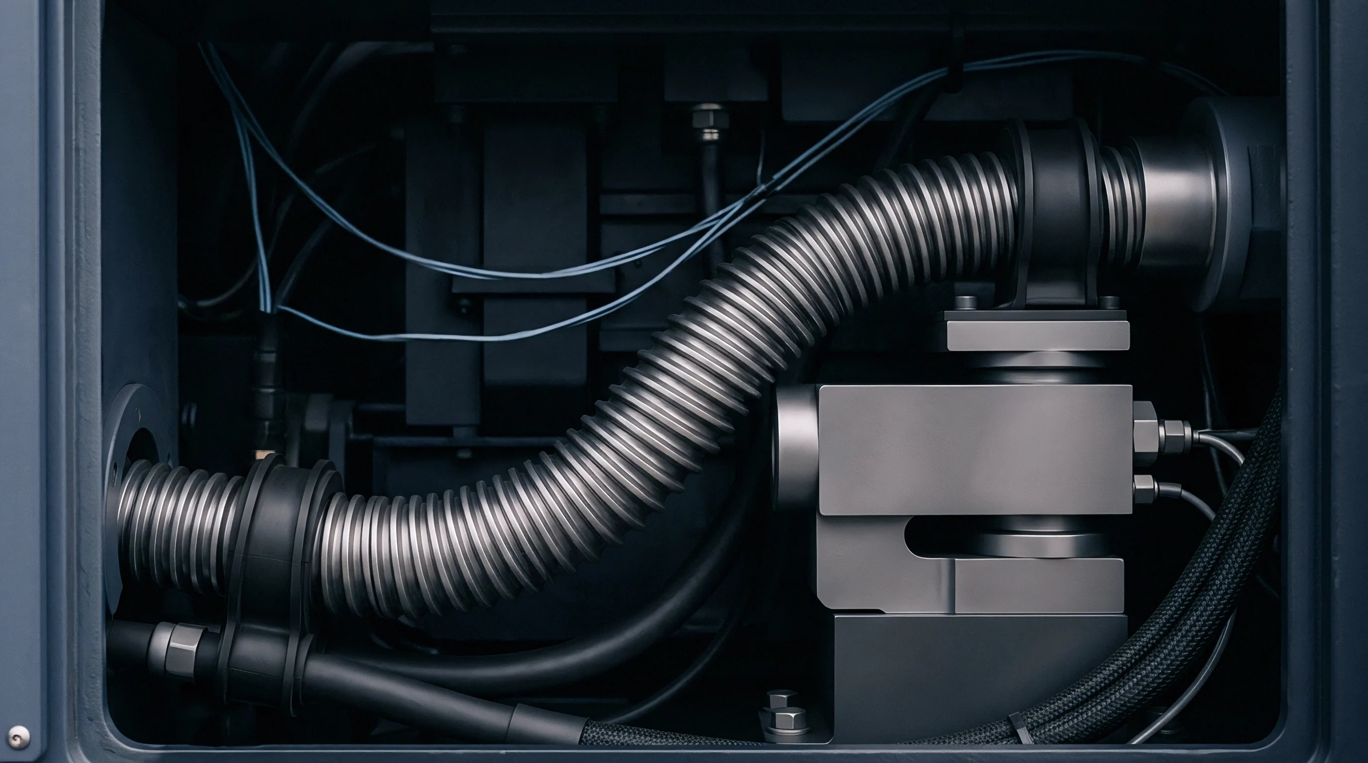
Compressed air distribution systems suffer from systemic pressure degradation when piping networks are sized solely for mean flow velocities. Standard sizing charts based on friction tables assume laminar or moderately turbulent flow under continuous steady-state conditions. In active manufacturing plants, compressed air behaves as a compressible gas governed by non-linear thermodynamics, where local pressure drop scales with the square of flow velocity and inversely with the fifth power of internal pipe diameter.
Pneumatic line starvation develops rapidly during multi-machine production cycles. When air moves through headers at velocities exceeding thirty feet per second, turbulent friction destroys useful pressure head. Energy dissipates as heat along pipe walls, leaving insufficient dynamic pressure at point-of-use drops.
Restrictive quick-disconnect fittings, undersized filter-regulator-lubricator assemblies, and long flexible rubber hoses at machine connection points compound the problem.

Friction Modeling in Compressible Gas Networks
Calculating real pressure drop across industrial compressed air piping requires solving the Darcy-Weisbach equation adapted for compressible fluids, incorporating density changes along the piping length. The fundamental pressure loss ΔP across pipe length L is expressed as:
ΔP = fD · ( L / D ) · ( ρ · v2 / 2 )
Where fD is the Darcy friction factor, D is pipe inner diameter in feet, ρ is fluid density under actual operating pressure, and v is mean gas velocity in feet per second. In compressible systems operating at typical industrial pressures between 90 and 125 pounds per square inch gauge, we apply the modified empirical empirical formulation for air flow:
ΔP = ( fD · L · Qacfm2 · P1 ) / ( 144 · D5 · Rgas · T )
Where Qacfm represents actual cubic feet per minute, P1 is inlet absolute pressure in pounds per square inch, Rgas is the specific gas constant for dry air, and T is absolute temperature in Rankine. The non-linear relationship between diameter D and pressure drop illustrates why minor reductions in pipe sizing produce catastrophic losses: halving pipe diameter increases dynamic friction by a factor of thirty-two for identical volumetric mass flow.
Equivalent length calculations must include pipe fittings, valves, tees, and directional elbows. Every 90-degree standard elbow introduces friction equivalent to twenty to forty pipe diameters of straight run. A complex piping layout with twenty elbows, four gate valves, and three cross tees adds hundreds of feet of equivalent resistance to the physical pipe route.
- Header velocity limits maintain compressed air transit speeds below twenty feet per second during baseline production and thirty feet per second during peak transient coincidence.
- Loop distribution topology feeds machine drops from multiple directions simultaneously, cutting effective path length and halving localized flow velocity across main line segments.
- Point of use regulation sets drop pressures ten to fifteen pounds per square inch lower than primary header pressure, establishing a built-in energy buffer that dampens line oscillation.
- Component restriction auditing eliminates undersized needle valves, coiled polyurethane drop lines, and high-loss push-in connectors between headers and actuator manifolds.

Transient Pressure Dynamics across Machine Drops
Actuator cycle times depend directly on the differential pressure across the valve spool and cylinder ports. When upstream line pressure collapses during an exhaust-and-stroke sequence, air volume cannot enter the cylinder chamber fast enough to overcome mechanical seal friction and load inertia. Machine cycle times lengthen unpredictably, throwing tightly synchronized assembly operations out of phase.
Pneumatic line drop issues frequently masquerade as mechanical component wear. Maintenance teams regularly increase main compressor discharge setpoints to compensate for point-of-use pressure starvation. Raising central compressor generation pressure from 100 to 125 psig increases power consumption by twelve to fifteen percent across central utility compressors without resolving localized transient drops.
High discharge pressure accelerates artificial demand, causes excessive compressed air leakage across fittings, and subjects air treatment equipment to higher thermal and moisture loads.
| Nominal Pipe Size (Schedule 40) | Actual Inner Diameter (Inches) | Flow Rate (SCFM) | Air Velocity (FT/Sec) | Friction Loss per 100 FT (PSI) | Terminal Pressure at 200 FT (PSIG) |
|---|---|---|---|---|---|
| 1.0 Inch | 1.049 | 150 | 46.2 | 4.82 | 90.36 |
| 1.5 Inch | 1.610 | 150 | 19.6 | 0.62 | 98.76 |
| 1.5 Inch | 1.610 | 400 | 52.2 | 4.12 | 91.76 |
| 2.0 Inch | 2.067 | 400 | 31.6 | 1.18 | 97.64 |
| 3.0 Inch | 3.068 | 800 | 28.5 | 0.31 | 99.38 |
| 4.0 Inch | 4.026 | 1,500 | 31.2 | 0.24 | 99.52 |
Proper pneumatic design treats the distribution network as an active storage reservoir rather than a simple transmission conduit. Oversized rigid aluminum or smooth-bore stainless steel piping lowers friction factors, prevents scale buildup, and provides secondary air buffering capacity immediately adjacent to high-demand production cells.
Straight runs sized two nominal diameters above continuous requirements hold line velocity within laminar bands, eliminating pressure starvation across downstream tools.


Tank
Localized pneumatic storage decouples transient peak mass flow from the main supply header. Expecting central air compressors to ramp up instantly for sub-second demand spikes violates basic rotary screw physics; a variable speed compressor requires several seconds to spool up and build internal pressure. When twenty high-flow vacuum ejectors actuate simultaneously, the transient air must emerge from accumulated storage located immediately beside the point of consumption.
Storage tanks operate as pneumatic capacitors. Sizing these vessels requires precise mathematical integration of the discharge profile, cycle duration, and permissible differential pressure drop. When storage volume is undersized, line pressure plummets during peak actuation, starving the tooling.
When storage volume is oversized without proper check valves, the tank draws excessive charging current from the primary distribution header during post-cycle recovery, starving adjacent production cells.

Mathematical Sizing of Dedicated Surge Vessels
Calculating the required secondary receiver tank volume Vtank in cubic feet depends on the peak transient air demand rate, baseline supply rate, event duration, and allowable pressure decay:
Vtank = /
Where Qdemand is the peak transient consumption rate in standard cubic feet per minute, Qsupply is the continuous flow entering the receiver from the primary header, tevent is the duration of the transient demand burst in minutes, Patm is atmospheric absolute pressure (14.7 psia at sea level), and ΔPallowed is the maximum permissible pressure drop in pounds per square inch across the receiver vessel during the event cycle.
Consider an automated bagging machine demanding 600 SCFM for a 4.0-second burst cycle, supplied by an upstream drop line restricted to 150 SCFM. The local process requires maintaining minimum delivery pressure at 85 psig from a primary line running at 100 psig, setting ΔPallowed to 15 psi. Converting event time to minutes yields tevent = 4 / 60 = 0.0667 minutes.
Applying the sizing relationship:
Vtank = / 15 = 441.22 / 15 = 29.41 text{ cubic feet}
Converting cubic feet to liquid gallons (using 7.4805 gallons per cubic foot) establishes a minimum vessel capacity of 220 gallons. Installing a standard 240-gallon receiver tank adjacent to the bagging apparatus completely buffers the transient spike, eliminating line pressure decay across adjacent machinery.

Is Receiver Volume Decoupled from Header Velocity?
Receiver effectiveness depends entirely on piping arrangement and flow control orientation. Connecting a surge tank inline without reverse-flow prevention or flow restricting orifices permits downstream tooling to pull unrestricted flow from both the tank and the upstream header simultaneously. High velocity transients still propagate backward into the primary distribution loop.
Decoupling requires dedicated check valves and calibrated metered refill circuits. A non-return check valve installed upstream of the secondary receiver ensures stored air flows exclusively toward the intermittent load. A flow-restricting needle valve or fixed orifice plate installed on the receiver bypass line limits the recharge rate during post-event recovery, flattening the demand profile observed by the main utility header.
Point of use air receivers installed without upstream non return check valves pull twenty percent of their recharge volume directly out of adjacent machine lines during sudden pressure transients.
Electrical power distribution utilizes parallel buffering architectures through capacitive uninterruptible power systems and ultra-capacitor storage banks. For high-power pulsed loads like resistance welding machines or heavy servo presses, localized capacitive storage or active harmonic filters compensate reactive currents in real time, injecting dynamic kilovars within five milliseconds of load engagement.
The operational balance between storage capacitance and recharge kinetics governs plant stability. The open engineering question remains how closely dynamic buffer recharge cycles can be synchronized with master PLC scan networks before communication latency and sensor drift induce resonant pressure and voltage hunting across interconnected manufacturing cells.


Switch
Coordinated load staging and control integration prevent simultaneous peak utility demand from crashing factory infrastructure. Uncontrolled concurrent operation represents an operational failure of production scheduling and control logic. When electrical substations and air compressor rooms run near thermal and volumetric limits, plant engineers can avoid multi-million-dollar utility expansion projects by implementing deterministic interlocks across automation software.
Industrial communication networks enable millisecond-level scheduling of high-draw operations. Fieldbus architectures like EtherCAT, Profinet, and Ethernet/IP support prioritized messaging and time-slotted execution. By interleaving the start sequences of high-inrush electric motors and staggering the actuation strokes of high-volume pneumatic tooling, control systems distribute peak utility demand evenly across time without reducing overall line throughput.

Deterministic Load Staggering Protocols
Implementing software-driven utility management requires mapping machine cycle profiles into clear operational priority tiers. Critical process steps receive immediate utility allocation, while non-critical indexing moves and charging cycles wait for available capacity windows.
Staggering motor starts eliminates additive locked-rotor current spikes. Direct-on-line induction motors draw peak inrush current for two to eight hundred milliseconds during initial magnetic field establishment and rotor acceleration. Programming a simple four-hundred-millisecond stagger delay between consecutive motor start commands on a major pumping bay reduces total starting current from thousands of amperes down to the baseline inrush of a single unit superimposed on running load.
- Baseline utility telemetry qualification establishes high-speed electrical and pneumatic logging across all primary distribution drops to identify overlapping peak transient vectors.
- Deterministic state scheduling execution assigns distinct scan-cycle start windows within programmable logic controller software to prevent synchronized valve manifold firing.
- Electronic soft starter deployment replaces mechanical motor contactors with silicon-controlled rectifier soft starters or variable frequency drives configured for controlled current-limit ramping.
- Dynamic pressure feedback integration reads local receiver vessel pressure and holds secondary machine cycles until pneumatic storage recovers to safe operating thresholds.

Commercial Specifications and Acceptance Criteria
Protecting capital expenditure during facility scale-up requires writing explicit dynamic utility performance tolerances into machine procurement contracts and facility build specifications. Standard vendor contracts typically state utility requirements as static average numbers, shifting financial responsibility to the buyer when equipment operation destabilizes plant utility grids.
Procurement documents must mandate maximum permissible transient current draw, minimum dynamic power factor, and maximum instantaneous pneumatic consumption rates. Acceptance testing protocols at the machinery builder facility must verify performance under fully loaded production conditions with high-speed power analyzers and inline flow meters attached.
| Utility Parameter | Standard Static Clause | Enforceable Dynamic Specification | Test Verification Method |
|---|---|---|---|
| Electrical Inrush | Rated: 480V, 3-Phase, 100A | Peak inrush ≤ 250% FLA for ≤ 100 ms; Power Factor ≥ 0.85 during start | Class A Power Quality Analyzer (IEC 61000-4-30) |
| Voltage Sag Immunity | Operational: 480V ± 10% | Continuous operation through SEMI F47 sag curve (50% depth for 200 ms) | Programmable AC Sag Generator Source |
| Peak Pneumatic Flow | Consumption: 50 SCFM Average | Instantaneous flow ≤ 120 SCFM; Pulse duration ≤ 1.5 seconds | High-Speed Thermal Mass Flow Meter (10 ms log) |
| Allowable Pressure Drop | Supply: 90 to 100 PSIG | Point-of-use pressure drop ≤ 5 PSI during full concurrent actuation | Piezoresistive Transducer at Tooling Manifold |
Explicit utility qualification standards belong directly in equipment master supply agreements. Section 4.3 of the standard capital equipment schedule states that equipment causing a secondary distribution voltage sag greater than four percent of nominal bus voltage, or a pneumatic header pressure drop exceeding eight pounds per square inch for longer than fifty milliseconds, fails site acceptance testing and requires vendor-funded power quality mitigation and accumulator installation before commercial handover.